(Non)equilibrium Green functions
Green functions describe the propagation of many-body states of added or removed particles. For these quantities exists a systematic diagrammatic perturbation expansion, both for equilibrium and nonequilibrium systems. From the Green functions a wealth of experimental data can be obtained. A brief introduction in this topic with further references can be found below. My research in this area is mainly concerned with
- Propagation of the Kadanoff-Baym equations
- Variational action functionals
- Connections with time-dependent density functional theory
The Kadanoff-Baym equations determine the time-evolution of the Green function. The variational action functionals provide a way a obtain good total energies from non-selfconsistent Green functions and to generate time-dependent density functionals within density-functional theory.
A brief introduction to (non)equilibrium Green functions
The Keldysh-Schwinger time-contour
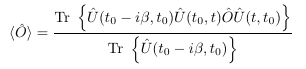
The Keldysh-Schwinger contour is a convenient bookkeeping device which allows you to derive simple expressions within nonequilibrium Green function theory in compact form. If you are familiar with equilibrium Green function theory then this contour is the only new thing that you need to learn. All expressions from equilibrium Green function theory remain valid within the nonequilibrium theory by a simple replacement of the time-integrals with a contour integral. The contour arises from the following simple considerations (for a more detailed introductions see [ 1 , 2 ]): From equilibrium quantum statistics we know that the expectation value of an operator Ô is given by:
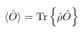
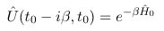
where the statistical operator is defined as
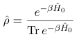
and where H0 is the (time-independent) Hamiltonian of the system. If we switch on an external field at time t0, the expectation value will be time-dependent for times t > t0 and given by
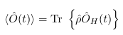
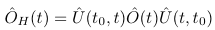
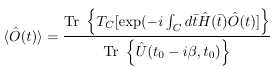
and therefore we can write the time-dependent expectation value equivalently as
If we read this expression from right to left then we note the following: We first evolve the system from time t0 to time t after which we act with the operator Ô. Then we propagate the system from time t back to t0. And then we finally propagate parallel to the imaginary axis from time t0 to time t0-iβ . This process can be described conveniently using a contour in the complex time plane and a time-ordering defined along the contour. The time-dependent expectation value then attains the form
where the time-contour has the following form:
For a more detailed introduction we again refer to [ 1 , 2 ]
Definition of the Green function
The one-particle Green function is defined as
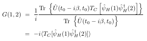
i.e. it is a contour-ordered product of a particle creation and annihilition field operator. Depending on whether t1 is larger or smaller than t2 on the contour the Green function describes the propagation of an added particle (i.e. an N+1 -body system) or a removed particle (N-1 - body system). The corresponding particle and hole propagators are denoted as G>(1,2) and G<(1,2). where we introduced for a space-time point the short notation 1=x1t1. The time-contour ordering operator TC appears naturally in the definition of the Green function as a consequence of the appearance of this operator in the time-evolution operator Û . From the Green function a wide variety of measurable quantities can be obtained such as the time-dependent particle and current densities, the ionization energies and electron affinities, the total energy and the excitation energies of the system and in general any expectation value of a one-body operator.
Kadanoff-Baym equations
The Kadanoff-Baym equations describe the time evolution of the two-time Green functions. They form a set of integro-differential equations. If the initial state of the system is an equilibrium state then the Kadanoff-Baym equations are solved in two steps. First the equations for the equilibrium Green functions are solved on the imaginary time axis. Subsequently a realtime propagation is carried out. A typical example of one of the Kadanoff-Baym equations is the following:
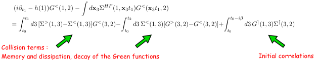
The right hand side of this equation contains the so-called collision terms that describe the correlations between the particles. These collision terms act as memory kernels, i.e. they involve integrations over earlier times. If we put t1 = t2 = 0 then the only term surviving on the right hand side is the last one. This is the term that describes the initial correlations in the equilibrium case and arises from the propagation along the imaginary time axis. The important quantity in the memory kernels is the self-energy Σ[G] which is a functional of the Green function G. This functional can be expressed pictorially in terms of Feynman diagrams as in the figure below In such diagrams every directed solid line represents a Green function and every wiggly line the Coulomb interaction connecting two space-time points. All the internal points of the diagram must be integrated over all space and all times on the contour.
Variational action functionals
Connections with time-dependent density-functional theory
References
- 1. R.van Leeuwen and N.E.Dahlen
- Introduction to Nonequilibrium Green Functions
- L.Kadanoff and G.Baym
- Quantum Statistical Mechanics Wiley (1960)
- M.Bonitz
- Quantum Kinetics, Teubner
- P.Danielewicz
- Quantum Theory of Nonequilibrium Systems,
Annals of Physics (1984)