Point-to-point focusing quadrupole doublet

In this example we build a system of two quadrupoles. The quadrupole fields are fitted to yield a point-to-point focusing quadrupole doublet system.

An optical system is point-to-point focusing if it images ions from one source point to a one image point. This means that the direction of the particle does not change the position at the image plane. In the first order this is true if the matrix elements (x|a) and (y|b) are zero in the system transfer matrix (remember \(a=\tan(\alpha)\) and \(b=\tan(\beta)\), where \(\alpha=v_x/v_z\) and \(\beta=v_y/v_z\)).

The overall procedure for this kind of task is:

• Build the optical system.

• Define the minimization function.

  • Set the new parameters (in this case the quadrupole fields).

  • Rebuild the system.

  • Read the relevant system transfer matrix coefficients.

  • Sum up the squares of the (x|a) and (y|b) and return this.

• Use standard minimization driver from scipy. This runs the defined minimization function until the minimum value has been found.

• Plot or use the results.

Importing the modules

In addition to previous example we need minimize from scipy.optimize.

import numpy as np
from scipy.optimize import minimize
import sys
sys.path.append('..')
import piol

Defining the parameters

Although the parameters like quadrupole radius or drift lengths can be defined in the call when the optical element is created usually better practice is to list the system parameters in the beginning of the file. This makes it much easier to change the system. Remember to add comments for all parameters!

# General parameters for this system
order  = 1     # order of transfer matrices in calculations
G0     = 0.05  # radius of both quadrupoles
Qlen   = 0.4   # Lenght of both quadrupoles
DLQ1Q2 = 0.1   # Drift length between the quadrupoles

# Initial values for the focusing powers in the quadrupoles. The field
# in Teslas is focusing power multiplied by the magnetic rigidity
Qf1    =  0.3 # +0.4243 would be correct for point-to-point
Qf2    = -0.6 # -0.4243 would be correct for point-to-point

# Creating a reference particle of 50 MeV, 100 u, 18 e.
refple = piol.ReferenceParticle(energy=50e6,mass=100,charge=18)
Brho = refple.magneticRigidity()
print( "Magnetic rigidity is {} Tm".format( Brho ) )

The fit is done in first order so there is no need for higher order here. However, after the fit one might be interested to increase the order to see the aberrations.

The magnetic quadrupole element requires magnetic field on poles in Teslas. However, the required field will be proportional to the magnetic rigidity of the reference particle and therefore changes if the reference particle changes. The more useful way is to define the strength of the quadrupole as focusing power which is the field divided by the magnetic rigidity. This is roughly the same is inverse of the focusing length. The unit of it is 1/lenght.

Building the system

Following step is to create the optical elements and pack those into a ElementStack. The variables pointing to quadrupoles, Q1 and Q2, are needed to access the fields during the minimization.

The function call writeFringeFields(force=True) gives PIOL permission to overwrite the GICOSYFF.DAT file before it asks transfer matrices from GICOSY program. You might want to backup that file first if you are using GICOSY without PIOL.

See the use of maxSAdvance=10 when the quadrupoles are defined. This ensures that the quadrupole is handled with one transfer matrix (since the length is less than 10 meters). This will speed up the minimization and do not have any effect on results since the full transfer matrix of the system does not depend on the number of transfer matrixes used for an element.

# Creating the elements in the system.
# Forcing the piol to overwrite GICOSYFF.DAT file.
piol.writeFringeFields(force=True)  
Source = piol.GeneralParticleSource(
    100,
    ('x',piol.Uniform(-1e-4,1e-4)),('a',piol.Uniform(-50e-3,50e-3)),
    ('y',piol.Uniform(-1e-4,1e-4)),('b',piol.Uniform(-20e-3,20e-3)),('t',0),
    ('m',refple.mass),('K',refple.energy),('q',refple.charge) )
DL1    = piol.GICOSYDrift( refple, 0.6, maxSAdvance=10, order=order )
Q1     = piol.Quadrupole( refple, 'magnetic', Qlen, Qf1*Brho, G0, maxSAdvance=10,
                          order=order)
DLQ1Q2 = piol.GICOSYDrift( refple, DLQ1Q2, maxSAdvance=10, order=order )
Q2     = piol.Quadrupole( refple, 'magnetic', Qlen, Qf2*Brho, G0, maxSAdvance=10,
                          order=order)
DL2    = piol.GICOSYDrift( refple, 0.6, maxSAdvance=10, order=order )

system = piol.ElementStack(name='qdoublet')
system.elements.append( Source )
system.elements.append( DL1 )
system.elements.append( Q1 )
system.elements.append( DLQ1Q2 )
system.elements.append( Q2 )
system.elements.append( DL2 )

Defining the function be minimized

The driver of the minimization will call this function with different parameter values. The parameters are varied until the minimum of the return value is found. Our return value is \((x|a)^2+(y|b)^2\) i.e. the squared sum of the first order transfer coefficients which should vanish when the system is point-to-point focusing.

Function also prints the parameters and the squared sum for each evaluation.

See the code how the parameters are updated and how the coefficients of the total system transfer matrix is accessed.

# Defining the function to be minimized
def doubletForMimimize( x ):
    Q1.setParameter( 'field', x[0]*Brho )
    Q2.setParameter( 'field', x[1]*Brho )
    system.rebuild()
    sysmatrix = system.getTransferMatrix()
    x_a = sysmatrix.getCoefficient('x','a')
    y_b = sysmatrix.getCoefficient('y','b')
    fv = x_a**2 + y_b**2
    print( 'doubletForMimimize: {:8.5f} {:8.5f} {:12.4e} {:12.4e} {:12.4e}'.format(x[0],x[1],x_a,y_b,fv) )
    return fv

Running the minimization

The following code calls the scipy.minimize() with our function and finally prints the parameters yielding the minimum function value. The parameters are the focusing powers of the two quadrupoles.

doOptimization=True

x0=[Qf1,Qf2]
if doOptimization:
    res = minimize( doubletForMimimize, x0, method='Nelder-Mead' )
    print( res.success, res.x )
    if not res.success:
        raise Exception('Couldn\'t find the minimum')
    Qf1 = res.x[0]
    Qf2 = res.x[1]
    Q1.setParameter( 'field', Qf1*Brho )
    Q2.setParameter( 'field', Qf2*Brho )

# Split elements for smoother plot (max 5 cm with one matrix)
system.setSAdvance(0.05)
system.rebuild()

After the minimization the setSAdvance() method of our system is called to increase the number of transfer matrices. In this particular case the increase of the number of the transfer matrices do not change the precision of calculation at all. The only case it usually has effect on final coordinates is when the system contains physical obstacles. However, here this makes the plot of the trajectories much smoother.

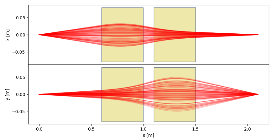
Transferring the particles and plotting

As in the previous example, one needs to create a driver, which collects the trajectories for ions, and transfer the particles through the system. Plottin of the trajectories can be easily made with piol.Plotter.

doOptimization=True

x0=[Qf1,Qf2]
if doOptimization:
    res = minimize( doubletForMimimize, x0, method='Nelder-Mead' )
    print( res.success, res.x )
    if not res.success:
        raise Exception('Couldn\'t find the minimum')
    Qf1 = res.x[0]
    Qf2 = res.x[1]
    Q1.setParameter( 'field', Qf1*Brho )
    Q2.setParameter( 'field', Qf2*Brho )

# Split elements for smoother plot (max 5 cm with one matrix)
system.setSAdvance(0.05)
system.rebuild()

Conclusions and testing

This example has shown that the piol library can be used with conventional python tools to minimize function values. In more advanced cases the objective function can even transfer particles and depend on higher order effects or transmission values.

One can try to change the system from point-to-point one to a point-to-parallel focusing or even having point-to-point focus in one direction and point-to-parallel focus in the other direction. Point-to-parallel can be obtained by changing the function to be minimized to \((a|a)^2+(b|b)^2\). Test!

To see the effect of system.setSAdvance(0.05) on plot smoothness, one can disable this line or change the value.

The full example

# This example is documented in
# ../docs/source/example_point_to_point_focusing_quadrupole_doublet.rst. Changing
# the line numbers will mess the example documentation. So, check the
# documentation if changing anything here.

# -- line 6 --
import numpy as np
from scipy.optimize import minimize
import sys
sys.path.append('..')
import piol
# -- line 12 --

# -- line 14 --
# General parameters for this system
order  = 1     # order of transfer matrices in calculations
G0     = 0.05  # radius of both quadrupoles
Qlen   = 0.4   # Lenght of both quadrupoles
DLQ1Q2 = 0.1   # Drift length between the quadrupoles

# Initial values for the focusing powers in the quadrupoles. The field
# in Teslas is focusing power multiplied by the magnetic rigidity
Qf1    =  0.3 # +0.4243 would be correct for point-to-point
Qf2    = -0.6 # -0.4243 would be correct for point-to-point

# Creating a reference particle of 50 MeV, 100 u, 18 e.
refple = piol.ReferenceParticle(energy=50e6,mass=100,charge=18)
Brho = refple.magneticRigidity()
print( "Magnetic rigidity is {} Tm".format( Brho ) )
# -- line 30 --

# -- line 32 --
# Creating the elements in the system.
# Forcing the piol to overwrite GICOSYFF.DAT file.
piol.writeFringeFields(force=True)  
Source = piol.GeneralParticleSource(
    100,
    ('x',piol.Uniform(-1e-4,1e-4)),('a',piol.Uniform(-50e-3,50e-3)),
    ('y',piol.Uniform(-1e-4,1e-4)),('b',piol.Uniform(-20e-3,20e-3)),('t',0),
    ('m',refple.mass),('K',refple.energy),('q',refple.charge) )
DL1    = piol.GICOSYDrift( refple, 0.6, maxSAdvance=10, order=order )
Q1     = piol.Quadrupole( refple, 'magnetic', Qlen, Qf1*Brho, G0, maxSAdvance=10,
                          order=order)
DLQ1Q2 = piol.GICOSYDrift( refple, DLQ1Q2, maxSAdvance=10, order=order )
Q2     = piol.Quadrupole( refple, 'magnetic', Qlen, Qf2*Brho, G0, maxSAdvance=10,
                          order=order)
DL2    = piol.GICOSYDrift( refple, 0.6, maxSAdvance=10, order=order )

system = piol.ElementStack(name='qdoublet')
system.elements.append( Source )
system.elements.append( DL1 )
system.elements.append( Q1 )
system.elements.append( DLQ1Q2 )
system.elements.append( Q2 )
system.elements.append( DL2 )
# -- line 56 --

# -- line 58 --
# Defining the function to be minimized
def doubletForMimimize( x ):
    Q1.setParameter( 'field', x[0]*Brho )
    Q2.setParameter( 'field', x[1]*Brho )
    system.rebuild()
    sysmatrix = system.getTransferMatrix()
    x_a = sysmatrix.getCoefficient('x','a')
    y_b = sysmatrix.getCoefficient('y','b')
    fv = x_a**2 + y_b**2
    print( 'doubletForMimimize: {:8.5f} {:8.5f} {:12.4e} {:12.4e} {:12.4e}'.format(x[0],x[1],x_a,y_b,fv) )
    return fv
# -- line 70 --

# -- line 72 --
doOptimization=True

x0=[Qf1,Qf2]
if doOptimization:
    res = minimize( doubletForMimimize, x0, method='Nelder-Mead' )
    print( res.success, res.x )
    if not res.success:
        raise Exception('Couldn\'t find the minimum')
    Qf1 = res.x[0]
    Qf2 = res.x[1]
    Q1.setParameter( 'field', Qf1*Brho )
    Q2.setParameter( 'field', Qf2*Brho )

# Split elements for smoother plot (max 5 cm with one matrix)
system.setSAdvance(0.05)
system.rebuild()
# -- line 89 --

# -- line 91 --
driver = piol.Driver()
system.transfer(driver)

plotter = piol.Plotter()
plotter.plotTrajectories(system, driver, kind='lines')
plotter.show()
# -- line 98 --