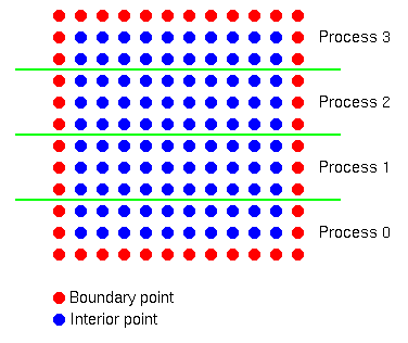
Any numerical analysis text will show that iterating
while (not converged) {y
  for (i,j)
    xnew[i][j] = (x[i+1][j] + x[i-1][j] + x[i][j+1] + x[i][j-1])/4;
  for (i,j)
    x[i][j] = xnew[i][j];
  }
will compute an approximation for the solution of Laplace's equation.
There is one last detail; this replacement of xnew with the average of the
values around it is applied only in the interior; the boundary values are
left fixed. In practice, this means that if the mesh is n by n, then the
values
x[0][j]
x[n-1][j]
x[i][0]
x[i][n-1]
are left unchanged. Of course, these refer to the complete mesh; you'll have to figure out what to do with for the decomposed data structures (xlocal).
Because the values are replaced by averaging around them, these techniques are called relaxation methods.
We wish to compute this approximation in parallel. Write a program to apply this approximation. For convergence testing, compute
diffnorm = 0;
for (i,j)
    diffnorm += (xnew[i][j] - x[i][j]) * (xnew[i][j] - x[i][j]);
diffnorm = sqrt(diffnorm);
You'll need to use MPI_Allreduce for this. (Why not use MPI_Reduce?)
Have process zero write out the value of diffnorm and the iteration count at
each iteration. When diffnorm is less that 1.0e-2, consider the iteration
converged. Also, if you reach 100 iterations, exit the loop. (The solution
of the test case should take a bit more than 90 iterations...)
Make the program collect the computed solution onto
process 0, which then writes the solution out (to standard output). You
might want to write the results out in a form that can be used for display
with tools like gnuplot or matlab, but this is not required. You may assume
that process zero can store the entire solution. Also, assume that each
process contributes exactly the same amount of data.
For simplicity, consider a 12 x 12 mesh on 4 processors.

The example solution uses the boundary values from the previous exercise; they are -1 on the top and bottom, and the rank of the process on the side. The initial data (the values of x that are being relaxed) are also the same; the interior points have the same value as the rank of the process. This is shown below:
-1 -1 -1 -1 -1 -1 -1 -1 -1 -1 -1 -1
 3  3  3  3  3  3  3  3  3  3  3  3
 3  3  3  3  3  3  3  3  3  3  3  3
 2  2  2  2  2  2  2  2  2  2  2  2
 2  2  2  2  2  2  2  2  2  2  2  2
 2  2  2  2  2  2  2  2  2  2  2  2
 1  1  1  1  1  1  1  1  1  1  1  1
 1  1  1  1  1  1  1  1  1  1  1  1
 1  1  1  1  1  1  1  1  1  1  1  1
 0  0  0  0  0  0  0  0  0  0  0  0
 0  0  0  0  0  0  0  0  0  0  0  0
-1 -1 -1 -1 -1 -1 -1 -1 -1 -1 -1 -1
Note that this is a very
You may want to use these MPI routines in your solution:
MPI_Init
MPI_Finalize
MPI_Send
MPI_Recv
MPI_Allreduce
MPI_Gather
MPI_Comm_size
MPI_Comm_rank