Approaches and Methods in Music Cognition & Perception: MIR
Pasi Saari - Martin Hartmann
Table of Contents
Starting to use MIRtoolbox
- Download MIRtoolbox from the following website:
https://www.jyu.fi/hum/laitokset/musiikki/en/research/coe/materials/mirtoolbox/Download
- follow the instructions, include e.g. “JYU Summer school in Human Sciences” in the “comments”
- get the recommended version (currently MIRtoolbox 1.7)
- In Finder, go to Downloads and unzip.
- Open the MATLAB folder (under /Applications, select the newest
MATLAB)
- Open “Set Path” dialog, remove any MIRtoolbox-related lines
- Select “Add with Subfolders…” and select Downloads/MIRtoolbox1.7
- Save and Close
- Test if MIRtoolbox works: In the Command Window, type
help mirtoolbox
Audio files that we will use during the workshop are available here: Audio files
Download the folder, unzip it, and set the current MATLAB working directory to the unzipped folder. MIRtoolbox also comes with a selection of audio files for test purposes, e.g. ragtime.wav. These are located in MIRtoolbox1.7/MIRToolboxDemos/ folder. We shall start by using the ragtime.wav, and then move onto more interesting song examples.
Basic Functionality of MIRtoolbox
Reading and processing an audio file (or mp3, ogg, etc.)
In order to analyse an audio file, it needs to be read into MIRtoolbox. It can be simply done by typing the following code, specifying the audio file name, and assigning it into a variable (a).
a = miraudio('ragtime.wav')
The read file can be played by
mirplay(a);
All files in a folder can be read by one line of code (your working directory needs to be in a folder containing some audio files).
a=miraudio('folder');
A more elaborate way to check the contents of a variable is to use the mirplayer. This will be later used to visualise musical features as well.
mirplayer(a)
Different parameters can also be specified for miraudio. One can for example trim the silence at the beginning and the end (’Trim’), specify the sampling rate (’Sampling’), or extract a certain clip of a file (’Extract’). The available options can be seen by typing
help miraudio
“help function-name” is useful for other functions as well.
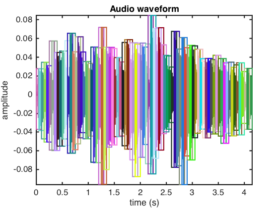
Frame decomposition of audio file
To extract musical features that evolve over time, one needs first to frame-decompose an audio file into shorter time frames. Features are then extracted for each frame separately. To decompose an audio file, run the following by specifying the frame length and overlap
a=miraudio('ragtime.wav');
frames = mirframe(a, .1, .5) % or frames = mirframe('ragtime.wav', .1, .5)
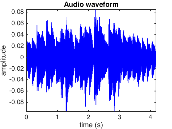
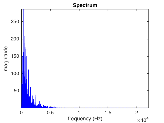
The frequency spectrum of audio
The sound energy at different frequencies can be extracted by computing the magnitude spectrum of audio waveform. This is done using the Fast Fourier Transform (FFT).
sp=mirspectrum(a) % or mirspectrum('ragtime.wav')
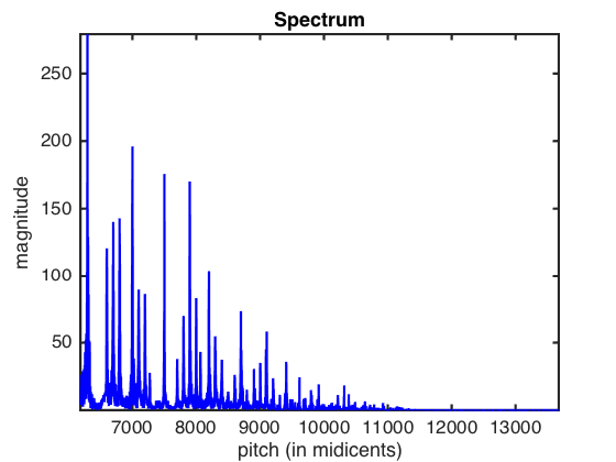
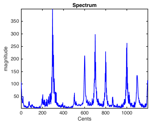
Frequency represented in cents (1/100 of a semitone):
sp=mirspectrum(a,'Cents')
Frequencies collapsed into one octave:
sp=mirspectrum(a,'Collapsed')
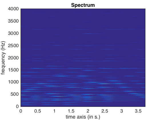
Spectrogram
Audio spectrogram is a time evolving representation of the audio spectrum. It can be obtained by computing the spectrum for a frame decomposed audio as follows:
sp=mirspectrum('ragtime.wav','Frame',.5,.1, 'Max',4000) % maximum frequency specified
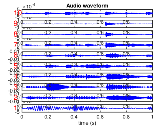
Filterbank decomposition
Filterbank decomposition separates an audio waveform into different frequency channels. It is useful when we want to extract fine-grained information from e.g. polyphonic audio where different frequency channels carry different instruments, rhythm, etc.
The default filter window is the gammatone.
fb = mirfilterbank('ragtime.wav','NbChannels',10,'Gammatone')
mirplay(fb)
Feature Extraction
A wide variety of musical/acoustic features can be extracted in MIRtoolbox. In the following some examples are given for different feature categories. Note that we are using the frame decomposition for most of the features in order to explore their temporal evolution.
First, let’s read a clip of a proper song (a better one than ragtime)
into a variable to make it faster to extract multiple features from it.
Set the Audio_files folder you downloaded as the working directory and
read a song.
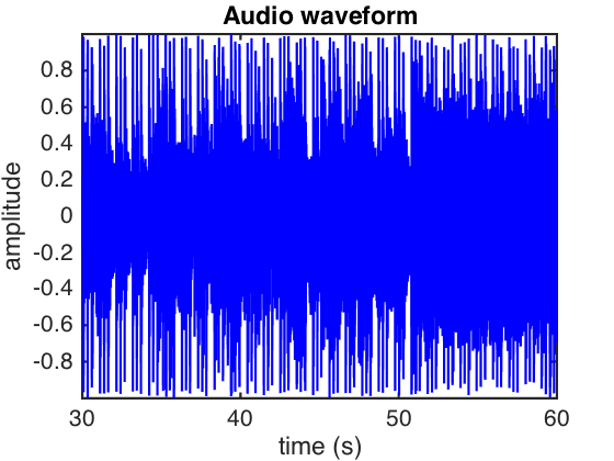
cd ~/Downloads/Audio_files/LongClips/ % or a similar path
n = miraudio('nirvana.mp3','Extract',30,60)
Dynamics
RMS
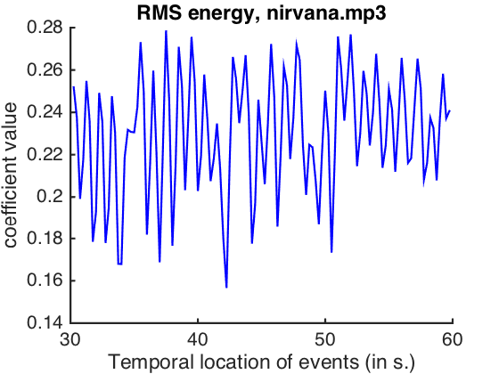
RMS is the computational energy (Root of the Mean Squared energy) of sound in audio time frames.
rms = mirrms(n, 'Frame',0.5,0.5)
mirplayer(rms)
Timbral features – how does the music sound?
Timbre is typically calculated from the spectrum or the spectrogram.
Brightness
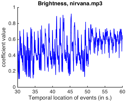
A basic timbral feature is the brightness, which is computed as the percentage of spectral energy that is above a specified cutoff frequency.
First, specify the cutoff frequency.
cutoff = 1500;
Brightness computation can be done in a single line as follows:
brightness = mirbrightness(n, 'Cutoff',cutoff)
In order to better understand what brightness means, we can compute it step by step and visualise it.
First, compute the spectrum and get its magnitude and the frequency of each magnitude in separate variables. The actual data for these are saved in a cell structure in {1}{1}, that denote {song}{channel}.
spectrum = mirspectrum(n)
magnitude = get(spectrum,'Magnitude');
frequency = get(spectrum,'Frequency');
frequency = frequency{1}{1};
magnitude = magnitude{1}{1};
Compute the brightness from the spectrum with the specified cutoff.
brightness = mirbrightness(spectrum, 'Cutoff',cutoff);
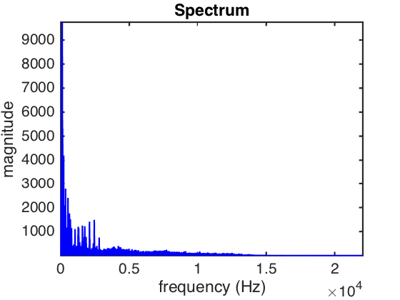
Visualise the brightness. The magnitudes are plotted at each frequency, and the plot is annotated.
plot(frequency, magnitude);
hold on; % hold the plot so we can annotate it
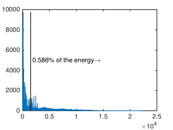
line([cutoff,cutoff],[0,max(magnitude)],'Color','k'); % line denoting the cutoff frequency
annotate = sprintf(' %0.3f%% of the energy\\rightarrow',mirgetdata(brightness)); % annotation text
text(cutoff,5000,annotate) % annotate with the text
The temporal evolution of brightness:
brightness = mirbrightness(n, 'Cutoff', 1500, 'Frame')
mirplayer(brightness)
Roughness
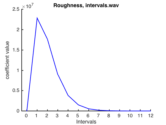
Roughness represents the sensory dissonance of sound. Partials of a complex sound, when close in frequency, create a beating phenomenon associated with the inability of human’s hearing system to separate them.
Roughly, roughness can be estimated by first computing the spectrum of sound, and then computing the distance between each pair of its frequency components. The more often the components with high enough amplitude tend to be within close proximity, the higher the roughness.
The following rather long example demonstrates this with intervals and pure sinusoid sounds. Note the difference in roughness with and without the overtones. Where is the beating?
Let’s first specify the input parameters. You may experiment with different parameter values.
semitones = 0:12; % specify the intervals
sampling_frequency = 44100;

basic_frequency = 440; % Hz (A)
tone_length = 2; % seconds
tone_time_instants = transpose(0:1/sampling_frequency:tone_length);
tone_mix = [0.5,0.5]; % both tones equally loud

n_overtones = 10;
overtones = 1:n_overtones; % multiples of the fundamental frequency

% both fundamental tones equally loud, higher overtones softer
tone_mix_overtones = 1./[2.^(1:n_overtones),2.^(1:n_overtones)];
Estimate roughness of intervals between simple sinusoids
waveform = []; % start with empty waveform

for n_semitones_higher = semitones

    % create the interval

    lower_tone = basic_frequency;
    % the higher tone in frequency
    higher_tone = basic_frequency * 2.^(n_semitones_higher/12);
    %combine the tones
    interval = [lower_tone,higher_tone];

    % represent interval as an audio waveform
    combined_tones = zeros(length(tone_time_instants),1); % reset
    for tone = 1:length(interval) % for both tones
        combine_this = tone_mix(tone)*sin(2.*pi.*interval(tone).*tone_time_instants);
        combined_tones = combined_tones + combine_this;
    end

    % append the interval to the end of the audio waveform
    waveform = [waveform;combined_tones];
end

% read to mirtoolbox
waveform = miraudio(waveform);
mirsave(waveform,'intervals.wav')

% Compute roughness
roughness = mirroughness('intervals.wav','Frame',2,1)

% visualise
ax = gca;
xlabel('Intervals');
ax.XTick=1:2:25;
ax.XTickLabel=0:12;
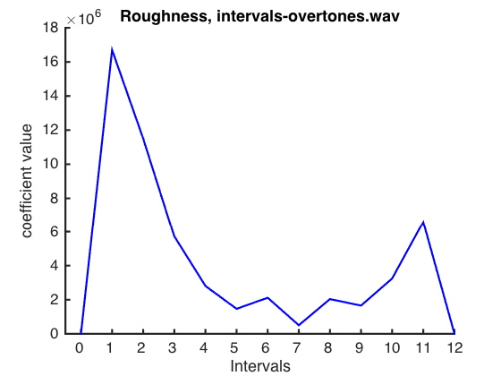
Here is the same type of estimation for sinusoids with added overtones.
waveform_overtones = []; % start with empty waveform

for n_semitones_higher = semitones

    % create the interval

    lower_tone = basic_frequency;
    % higher tone inluding the overtones
    lower_tone_overtones = lower_tone * overtones;
    % the higher tone in frequency
    higher_tone = basic_frequency * 2.^(n_semitones_higher/12);
    % higher tone inluding the overtones
    higher_tone_overtones = higher_tone * overtones;
    %combine the tones
    interval_overtones = [lower_tone_overtones,higher_tone_overtones];

    % represent interval as an audio waveform
    combined_tones_overtones = zeros(length(tone_time_instants),1); % reset
    for overtone = 1:length(interval_overtones) % for both tones
        combine_this = tone_mix_overtones(overtone)*sin(2.*pi.*interval_overtones(overtone).*tone_time_instants);
        combined_tones_overtones = combined_tones_overtones + combine_this;
    end

    % append the interval to the end of the audio waveform
    waveform_overtones = [waveform_overtones;combined_tones_overtones];

end

% read to mirtoolbox
waveform_overtones = miraudio(waveform_overtones);
mirsave(waveform_overtones,'intervals-overtones.wav')

% Compute roughness
roughness_overtones = mirroughness('intervals-overtones.wav','Frame',2,1)

% visualise
ax = gca;
xlabel('Intervals');
ax.XTick=1:2:25;
ax.XTickLabel=0:12;
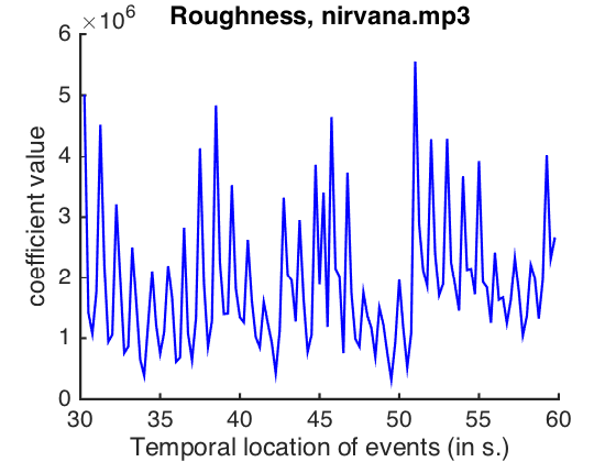
Roughness computed for the frame-decomposed audio:
roughness = mirroughness(n, 'Frame',0.5,0.5)
mirplayer(roughness)
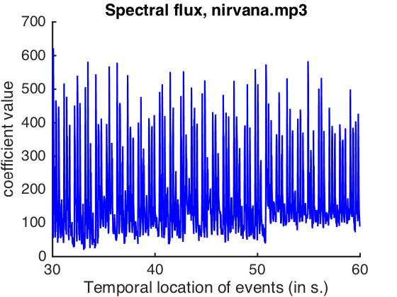
Spectral flux
Spectral flux represents how much discrepancy there is in the spectrum between adjacent time frames.
spectralflux = mirflux(n, 'Frame')
mirplayer(spectralflux)
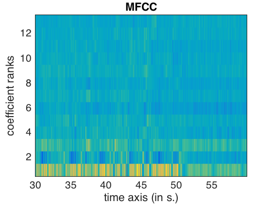
MFCC
Mel-Frequency Cepstral Coefficients model the human auditory response (Mel scale). They can be used for summarising the timbral characteristics, and are useful for different music classification tasks such as music genre classification and auto-tagging.
mfcc = mirmfcc(n,'Frame')
Collecting all together
Next we shall explore all of the features computed for the Nirvana song. The features may be collected together by assigning them into a structure as follows. Listen to the song using the mirplayer and try to relate the changes in the features to the changes in the song characteristics.
nirvana.rms = rms;
nirvana.spectralflux = spectralflux;
nirvana.brightness = brightness;
nirvana.roughness = roughness;
nirvana.mfcc = mfcc;
mirplayer(nirvana)
Rhythm
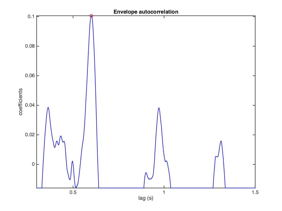
mirtempo
Tempo estimation can be performed by computing the autocorrelation of an amplitude envelope. Go to the LongClips folder and compute the global tempo value for ’yesterday.wav’:
[t1 t2] = mirtempo('yesterday')
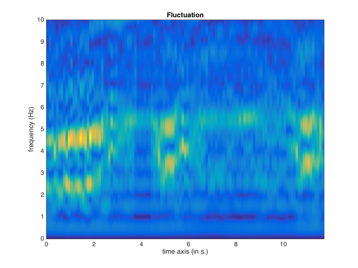
mirfluctuation
Fluctuation Patterns (Pampalk et al., 2002) is a psychoacoustics-based representation of rhythmic periodicities in the audio signal. It is obtained via estimation of spectral energy modulation over time at different frequency bands. Let’s compute fluctuation patterns for a spectrogram of ’czardas.wav’ and sum the obtained spectrum across bands. The result shows global rhythmic periodicity as a function of time.
mirfluctuation('czardas.wav','frame','summary')
mirpulseclarity
Get an estimation of the strength of the beat, or the relative importance of the regular pulsation. Let’s get the pulse clarity from the beginning of ’daftpunk’:
a = miraudio('daftpunk.mp3','Extract',0,2)
mirpulseclarity(a)
We can compare this estimation with the pulse clarity of other stimuli, such as ’yesterday.wav’ or ’singing.wav’
mireventdensity
Event density refers to the number of note onsets per second in the music. To obtain note onsets, peak detection can be applied to the amplitude envelope. Obtain the note onset density of ’basoon’. High values mean that there are many notes per second, and vice versa.
mireventdensity('basoon.wav')
Pitch
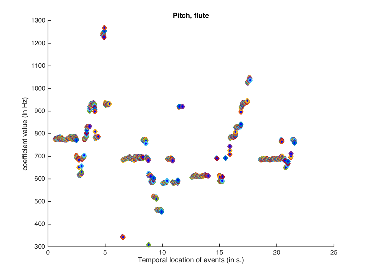
mirpitch
Obtain information about the pitch heights for ’flute.wav’ by computing an autocorrelation of a frame-decomposed signal:
mirpitch('flute.wav', 'Frame')
Tonality
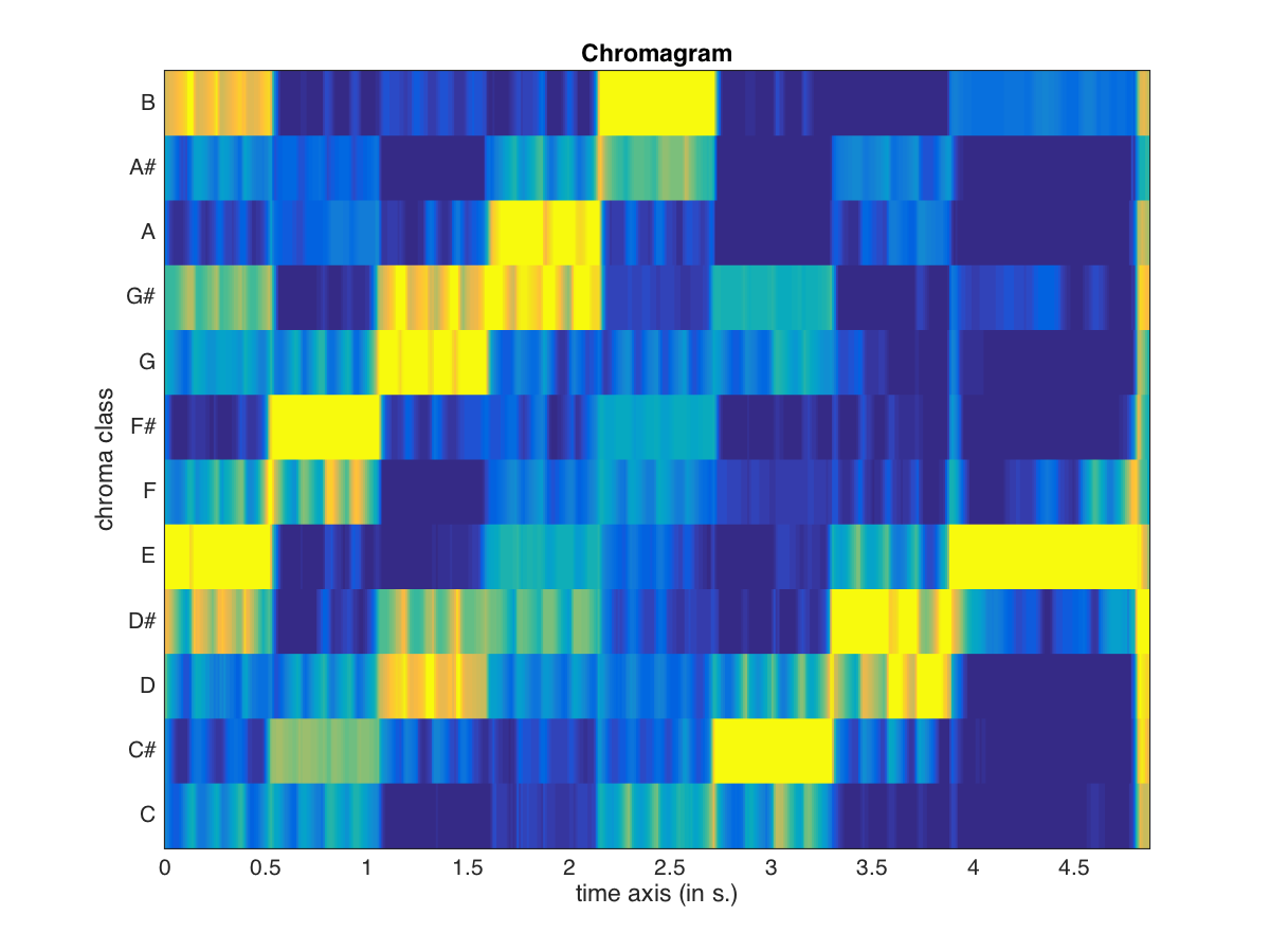
mirchromagram
The chromagram or Pitch Class Profile (Fujishima, 1999) describes the distribution of spectral energy along the 12 pitch classes. Let’s compute it for ’basoon.wav’:
mirchromagram('basoon.wav')
See the evolution of the pitch class profile over time with the ’Frame’ option:
mirchromagram('basoon.wav','Frame')
Chromagram is computed by default with 12 bins per octave, one per pitch class. We can add more bins to account for microtones, bent notes, etc.:
mirchromagram('basoon.wav','Frame','res',24)
Also the chromagram can be unwrapped to yield a representation of the signal for different pitch heights:
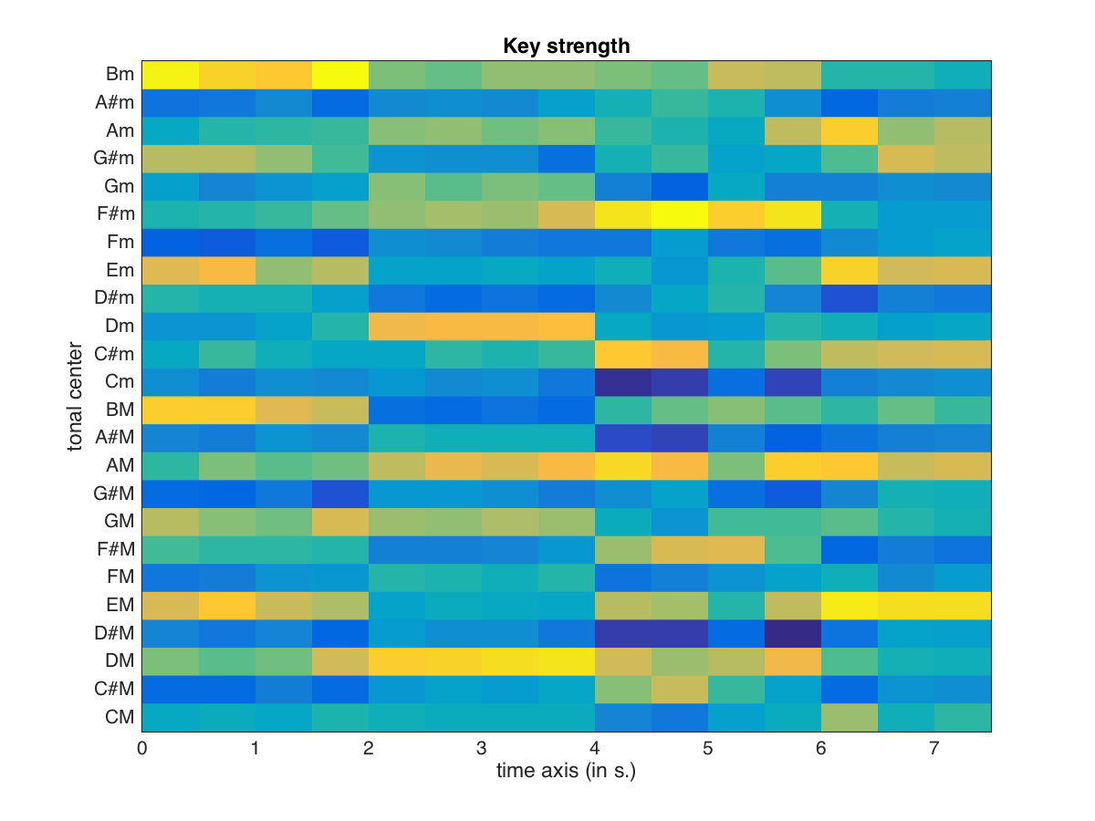
mirkeystrength
The Key Strength is computed as the correlation between the chromagram and the 24 key profiles obtained from empirical work by Krumhansl & Kessler (1982); you can listen to an example of the probe-tone sequences used in the experiments to obtain key profiles:
Let’s select the first 8 seconds of ’daftpunk’, apply frame decomposition using a window length of 1 s, and compute the likelihood of each key:
a = miraudio('daftpunk.mp3','extract',0,8,'frame',1);
mirkeystrength(a)
mirkey
mirkey finds the single most probable key based on the results of mirkeystrength.
[k,kc,ksp] = mirkey(a)
Structure
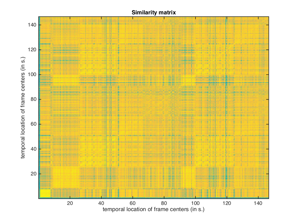
mirsimatrix
A self-similarity matrix (Foote, 1999) is a square matrix indicating the similarity between each possible pair of data points:

It can be computed in MIRToolbox via the mirsimatrix function, and it is computed by default from the spectrogram. Let’s extract MFCCs from ’nirvana’ and compute its similarity matrix:
m = mirmfcc('nirvana.mp3','frame')
s = mirsimatrix(m)
a = miraudio('daftpunk.mp3','extract',0,16,'frame',1);
k = mirkeystrength(a)
s = mirsimatrix(k)
Notice that the changes in the main diagonal are relevant to find segments in the piece, but other diagonals can provide information about repetitions in the music.
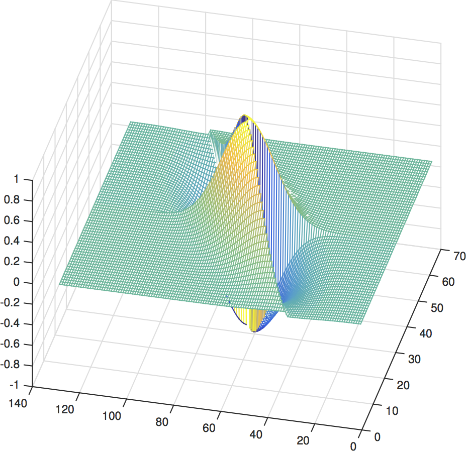
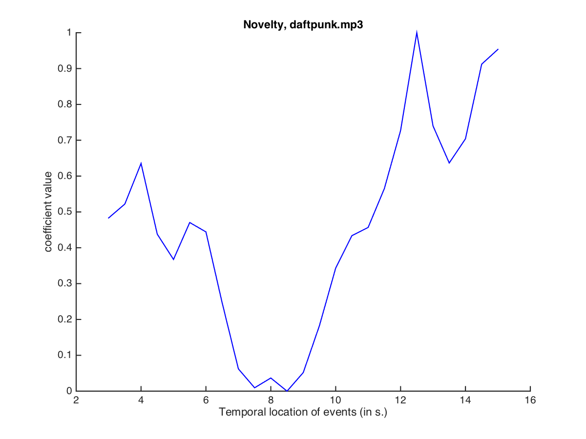
mirnovelty
The novelty-based approach (Foote, 2000) for structural segmentation involves the convolution between a Gaussian Checkerboard Kernel and a similarity matrix. Musical feature discontinuity with respect to a given temporal context will be represented as high novelty. Let’s compute a novelty curve for the similarity matrix obtained from the key strength of ’daftpunk’ using a kernel of 64 feature frames:
n = mirnovelty(s,'kernelsize',64)
Alternatively, the default strategy for mirnovelty in MIRToolbox (Lartillot et al., 2013) detects novelty taking into account the amount of homogeneity of the past segment and the amount of contrast between time points.
n2 = mirnovelty(s)
mirpeaks is a general-purpose function that can be used for peak picking in order to obtain segment boundaries from the novelty curves:
p = mirpeaks(n)
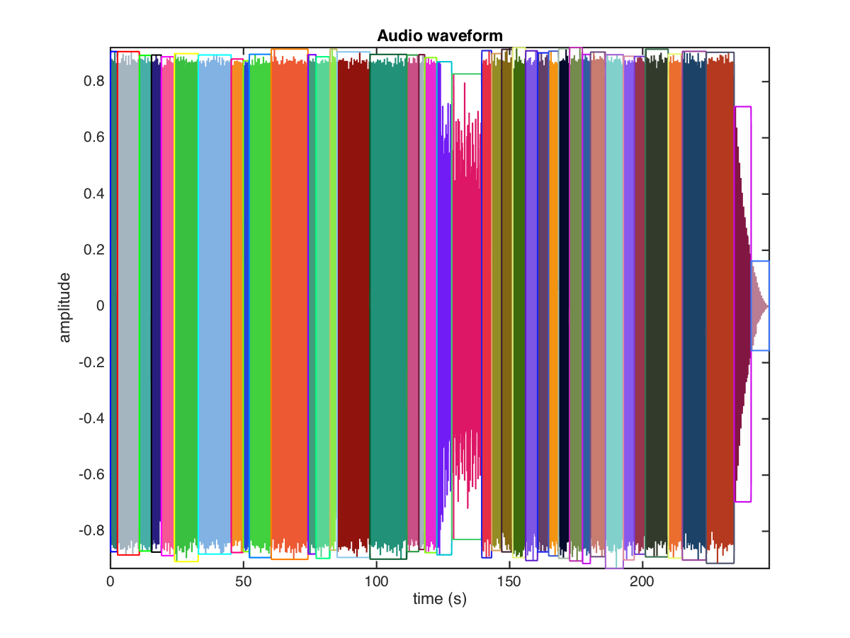
mirsegment
Peak locations can be used as an input together with a miraudio object for mirsegment. This will show us the proposed segmentation over the audio waveform:
a = miraudio('daftpunk.mp3');
c = mirkeystrength(a,'frame',3);
n = mirnovelty(c,'kernelsize',64);
p = mirpeaks(n);
s = mirsegment(a,p)
You can now listen to each segment stored in the variable s with mirplay.
Saving and Exporting
mirgetdata
mirgetdata can be used to obtain data from a mirtoolbox object for further computation in Matlab. For instance we can get the obtained peak locations:
mirgetdata(p)
We can also obtain feature data for a folder of music with mirgetdata. For instance, we can go to the ShortClips and compute brightness for the whole folder:
cd ~/Downloads/Audio_files/ShortClips/
a = miraudio('Folder');
b = mirbrightness(a)
g = mirgetdata(b)
This will return a global brightness value for each snippet of music. These values are sorted based on their respective file names. To make better sense of the results it is possible to use mirplay. We can sort different musical pieces based on their global brightness value and play the pieces in increasing order of brightness:
mirplay(a,'increasing',b)
mirsave
It is possible for some functions to save temporal data as a wave file. For instance, an amplitude envelope can be sonified using white noise and saved as a wave file:
e = mirenvelope('basoon.wav','frame')
mirsave(e)
We can also compute filterbank decomposition for an extract of ’daftpunk’ and save each frequency channel as a separate wave file:
a = miraudio('daftpunk.wav','extract',0,4.5,'middle')
fb = mirfilterbank(a)
mirsave(fb,'Channels',1)
mirexport
mirexport can be used to export statistical information of a result into a text file. For instance, we can use mirfeatures to compute a set of features from one or multiple files, and export statistics obtained from the features via mirexport:
f = mirfeatures('ragtime.wav')
mirexport('myfile.txt',f)
References
- Foote, J. (2000). Automatic audio segmentation using a measure of audio novelty. In IEEE International Conference on Multimedia and Expo, volume 1, pages 452–455. IEEE.
- Fujishima, T. (1999). Realtime chord recognition of musical sound: A system using common lisp music. In Proceedings of the International Computer Music Conference, volume 1999, pages 464–467.
- Krumhansl, C. L. and Kessler, E. J. (1982). Tracing the dynamic changes in perceived tonal organization in a spatial representation of musical keys. Psychological review, 89(4):334.
- Lartillot, O., Cereghetti, D., Eliard, K., and Grandjean, D. (2013). A simple, high-yield method for assessing structural novelty. In Luck, G. and Brabant, O., editors, Proceedings of the 3rd International Conference on Music & Emotion (ICME3), Jyväskylä, Finland.
- Lartillot, O. and Toiviainen, P. (2007). A Matlab toolbox for musical feature extraction from audio. In International Conference on Digital Audio Effects, pages 237–244, Bordeaux.
- Pampalk, E., Rauber, A., and Merkl, D. (2002). Content-based organization and visualization of music archives. In Proceedings of the tenth ACM international conference on Multimedia, pages 570–579. ACM.