Classification Demo
![]()
| Music Information Retrieval - MUSS1112 |
| October 13, 2017 |
| Martin Hartmann - martin.hartmann@jyu.fi |
1 Matlab
1.1 Genre classification with MIRToolbox
- We will perform musical genre classification using an audio data set that is included in the MIRToolbox installation (
MIRtoolboxDemos/folder). First, check the documentation for mirclassify in the MIRToolbox Users’ Manual. Go to the folder/Users/Shared/, you will find theMIRtoolbox/folder there. It includes the Manual and theMIRtoolboxDemos/folder. - The function mirclassify can be used with balanced data sets. The folder structure of the data set is important; there should be a subfolder for each class. The name of each subfolder will be used as a class label.
- mirclassify uses leave-one-out cross-validation classification: for a data set with n examples, it trains the data on n-1 examples and tests the data on the example which was left out. This process is repeated until the data is tested on all examples.
- Once you are in the
MIRToolbox/folder, you can navigate from there to the data set that we will use, which is located inMIRToolboxdemos/classif/. Listen to some of the musical examples to get an idea of the type of data that we will use for classification.
1.1.1 In Matlab
- Open Matlab and navigate to the
classif/folder.
1.1.2 Classification using global descriptors
- We can try a k-NN classification based on some features. For instance, mirmfcc (13 dimensions), mircentroid and mirzerocross:
mirclassify({mirmfcc('Folders'), mircentroid('Folders'), mirzerocross('Folders')})
- We now obtained a confusion matrix, a correct classification rate, and a figure illustrating the mean feature values for each musical example. Each row is a feature and each column is an example. Let’s try to make the figure a bit easier to read by adding a title:
title('Mean feature values of the dataset')
- To make the figure more clear, let’s add some labels.
xlabel('Musical example')
ylabel('Feature')
- The examples have been randomly permuted, but they are grouped by class. The features are ordered from top to bottom based on our call to mirclassify, so we can label them. The figure will not look perfect, but things will be easier to understand.
% Let's start with the 13 MFCCS
for k = 1:13, featlabels{k} = strcat('MFCC',num2str(k)), end
% Now we can add the other features
featlabels{end+1} = 'Spectral Centroid';
featlabels{end+1} = 'Zero-crossing Rate';
% Now we can add the feature labels
set(gca,'Ytick',1:15,'YTickLabel',featlabels)
1.1.3 Feature extraction with Design option
- Let’s try a different approach to feature extraction. This method will allow us to add labels to each miraudio object, which are required for other parts of this demo.
lb = [repmat({'bq'}, 1,13) repmat({'cl'}, 1,13) repmat({'md'}, 1,13) repmat({'rm'}, 1,13)];
a = miraudio('Design','label',lb);
f.rms = mirrms(a,'Frame');
f.mfcc = mirmfcc(a,'Frame');
f.brightness = mirbrightness(a,'Frame');
f.subband_flux = mirflux(a,'Subband');
f.chromagram = mirchromagram(a,'Frame');
- Now we will extract RMS, MFCCs, brightness, subband flux and chromagram:
e = mireval(f,'Folders')
- Since we used the ’frame’ option, we now have short-term features. We will compute the mean of each feature. We could compute other statistics as well. See mirmedian, mirstd, mirkurtosis, and mirskewness.
m = mirmean(e)
- Finally, we can classify using k-NN:
mirclassify({m.rms m.mfcc m.brightness m.subband_flux m.chromagram})
- Try modifying the features used, or using just one set of features, such as MFCCs or sub-band flux, and see whether you can find an improvement in the classification results.
- Homework: try to add a title, x axis and y axis labels, and feature labels. Remember that we have 13 MFCCs, 10 subband fluxes, and that the chromagram consists of 12 dimensions.
- Also, you can try using another value of k, for example:
mirclassify({m.rms m.brightness m.mfcc m.subband_flux m.chromagram},...
 'Nearest', 5)
- Did this reduce the generalization error?
1.2 Creating an ARFF file for Weka
- mirexport will export statistical information related with the computed short-term features:
cd ~/Downloads
mirexport('~/Downloads/test.arff',e)
- It is possible to export only certain statistical information. For example, we extracted feature means via mirmean and these values can be exported:
mirexport('~/Downloads/test_means.arff',m)
2 Weka
2.1 Download Weka
- Go to the Weka website –> (Getting Started) Download. –> Mac OS X
- Copy the content of the disk image into a folder, such as Downloads. Try to open the file that has the Weka icon.
- If you get an error, go to System Preferences –> Security & Privacy –> Open anyway
2.2 The ARFF viewer
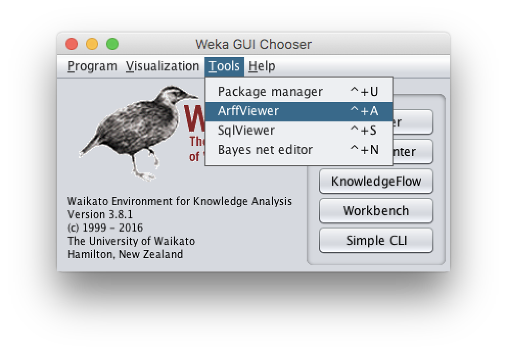
- This viewer allows you to load and manually edit your data set.
2.3 The Weka Explorer
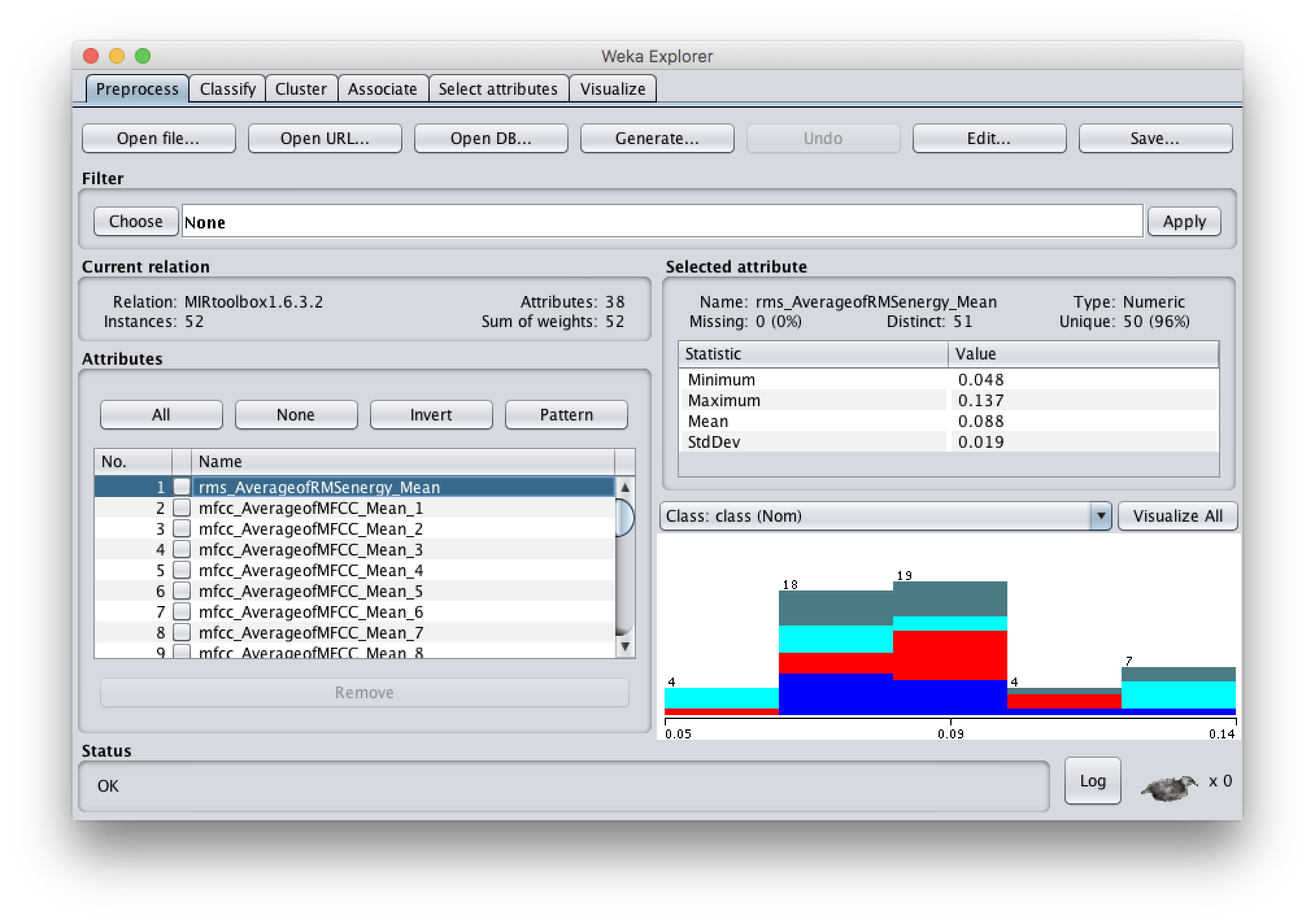
- The Explorer is useful for getting to know your data set and getting familiar with the available tools.
- In the Preprocess panel you can also load your dataset, and do more editing such as removal of attributes. You can explore for instance the range of values of your features, or how many missing feature values you have.
- One of the attributes is the class attribute: it shows, for example, if the dataset is balanced or not.
2.3.1 Filtering data
- We can try some of the data filtering options in Weka. Let’s choose to standardize (unsupervised -> attribute -> Standardize) the data so that each feature has a mean of 0 and SD of 1.
2.4 Classify Panel
- Let’s try k-NN classification, (IBk), this time in Weka. You can use cross-validation classification.
2.4.1 Interpretation of the output
The classifier output not only informs about the results, but it also records other detailed information about the classification, such as what classifier was applied, and what dataset was used.
2.4.2 Visualize classifier errors and margin
- The result list shows all the classifications that have been executed in the current Weka session. You can right-click on the last classification to visualize the classifier errors.
- In this visualization, each x indicates a correctly classified instance, whereas the squares indicate misclassifications.
- You can try clicking on one of the instances.
- From the result list, you can also take a look at the margin curve.
- You can also look at threshold curves for each class label of the dataset. Here you can compare several performance meassures.
2.5 Select attributes Panel
- Weka includes multiple attribute selection methods. We can try Filter attribute selection to eliminate redundant features that correlate with each other to reduce the number of dimensions and maybe even improve our classification results. Let’s use CfsSubsetEval attribute evaluator with the BestFirst search method for this.
- We can try saving the reduced data (right click in result list) and running the classification algorithm one more time and see whether there is an improvement in the results.
2.6 Other classifiers
- You can explore other classifiers and compare the obtained results. For example:
- A bayesian classifier, NaiveBayes
- SMO function, a support vector machine classifier
2.7 Other ways of running Weka schemes
- Finally, it is possible to set up more elaborate learning tasks using the Experimenter or the Knowledge Flow. Both are intrduced in the Weka Manual; you can find
WekaManual.pdfin the Weka installation folder. - Weka can also be run from the command line. Check out the Weka Primer for more information.